Easy methods to Estimate Pace with Pc Imaginative and prescient

Have you ever ever questioned how one can estimate the velocity of autos utilizing pc imaginative and prescient? On this tutorial, I’ll discover the complete course of, from object detection to monitoring to hurry estimation. 

Alongside the way in which, I confronted the challenges of perspective distortion and discovered tips on how to overcome them with a little bit of math!

This weblog put up incorporates brief code snippets. Comply with alongside utilizing the open-source pocket book we’ve ready, the place you’ll discover a full working instance. We’ve additionally launched a number of scripts appropriate with the most well-liked object detection fashions, which you will discover right here.

Object Detection for Pace Estimation

Let’s begin with detection. To carry out object detection on the video, we have to iterate over the frames of our video, after which run our detection mannequin on every of them. The Supervision library handles video processing and annotation, whereas Inference supplies entry to pre-trained object detection fashions. We particularly load the yolov8x-640 mannequin from Roboflow.

If you wish to be taught extra about object detection with the Inference, go to the Inference GitHub repository and documentation.

import supervision as sv
from inference.fashions.utils import get_roboflow_model mannequin = get_roboflow_model(‘yolov8x-640’)
frame_generator = sv.get_video_frames_generator(‘autos.mp4’)
bounding_box_annotator = sv.BoundingBoxAnnotator() for body in frame_generator: outcomes = mannequin.infer(body)[0] detections = sv.Detections.from_inference(outcomes) annotated_frame = trace_annotator.annotate( scene=body.copy(), detections=detections)

In our instance we used Inference, however you’ll be able to swap it for Ultralytics YOLOv8, YOLO-NAS, or some other mannequin. It’s worthwhile to change a couple of strains in your code, and try to be good to go.

import supervision as sv
from ultralytics import YOLO mannequin = YOLO("yolov8x.pt")
frame_generator = sv.get_video_frames_generator(‘autos.mp4’)
bounding_box_annotator = sv.BoundingBoxAnnotator() for body in frame_generator: consequence = mannequin(body)[0] detections = sv.Detections.from_ultralytics(consequence) annotated_frame = trace_annotator.annotate( scene=body.copy(), detections=detections)

Multi-Object Monitoring for Pace Estimation

Object detection isn’t sufficient to carry out velocity estimation. To calculate the gap traveled by every automotive we want to have the ability to monitor them. For this, we use BYTETrack, accessible within the Supervision pip package deal.

... # initialize tracker
byte_track = sv.ByteTrack() ... for body in frame_generator: outcomes = mannequin.infer(body)[0] detections = sv.Detections.from_inference(outcomes) # plug the tracker into an current detection pipeline detections = byte_track.update_with_detections(detections=detections) ...

If you wish to be taught extra about integrating BYTETrack into your object detection venture, head over to the Supervision docs web page. There, you’ll discover an end-to-end instance exhibiting how you are able to do it with totally different detection fashions.

Perspective Distortion in Distance Measurement

Let’s contemplate a simplistic strategy the place the gap is estimated based mostly on the variety of pixels the bounding field strikes.

Right here’s what occurs while you use dots to memorize the place of every automotive each second. Even when the automotive strikes at a constant velocity, the pixel distance it covers varies. The additional away it’s from the digital camera, the smaller the gap it covers.

Because of this, it will likely be very arduous for us to make use of uncooked picture coordinates to calculate the velocity. We want a strategy to remodel the coordinates within the picture into precise coordinates on the highway, eradicating the perspective-related distortion alongside the way in which. Luckily, we are able to do that with OpenCV and a few arithmetic.

Math Behind Perspective Transformation

To rework the attitude, we want a Transformation Matrix, which we decide utilizing the getPerspectiveTransform perform in OpenCV. This perform takes two arguments – supply and goal areas of curiosity. Within the visualization under, these areas are labeled A-B-C-D and A'-B'-C'-D', respectively.

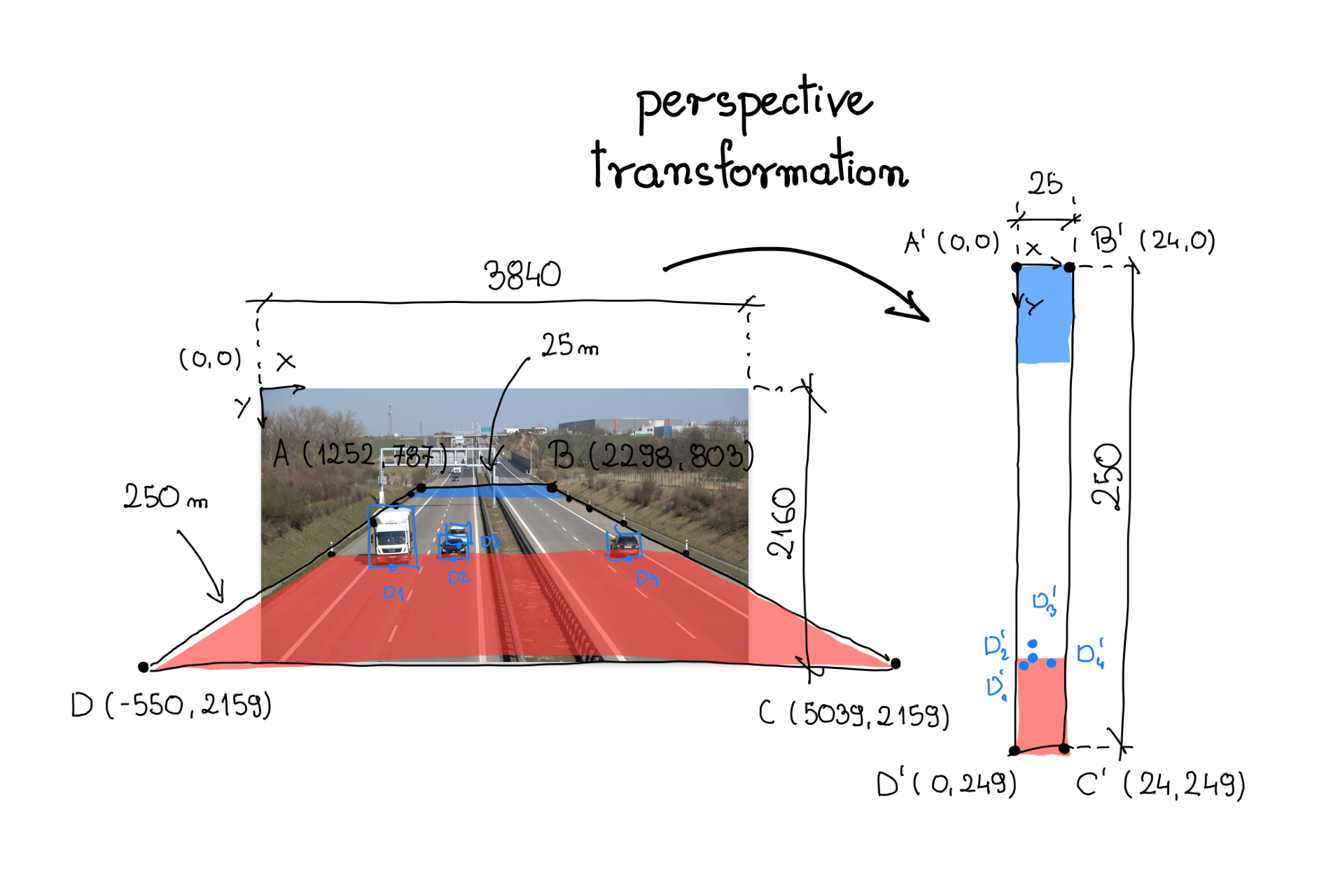
Analyzing a single video body, I selected a stretch of highway that may function the supply area of curiosity. On the shoulders of highways, there are sometimes vertical posts – markers, spaced each fastened distance. On this case, 50 meters. The area of curiosity spans the complete width of the highway and the part connecting the six aforementioned posts.

In our case, we’re coping with an expressway. Analysis in Google Maps confirmed that the world surrounded by the supply area of curiosity measures roughly 25 meters extensive and 250 meters lengthy. We use this info to outline the vertices of the corresponding quadrilateral, anchoring our new coordinate system within the higher left nook.

Lastly, we reorganize the coordinates of vertices A-B-C-D and A'-B'-C'-D' into 2D SOURCE and TARGET matrices, respectively, the place every row of the matrix incorporates the coordinates of 1 level.

SOURCE = np.array([ [1252, 787], [2298, 803], [5039, 2159], [-550, 2159]
]) TARGET = np.array([ [0, 0], [24, 0], [24, 249], [0, 249],
])

Perspective Transformation

Utilizing the supply and goal matrices, we create a ViewTransformer class. This class makes use of OpenCV’s getPerspectiveTransform perform to compute the transformation matrix. The transform_points methodology applies this matrix to transform the picture coordinates into real-world coordinates.

class ViewTransformer: def __init__(self, supply: np.ndarray, goal: np.ndarray) -> None: supply = supply.astype(np.float32) goal = goal.astype(np.float32) self.m = cv2.getPerspectiveTransform(supply, goal) def transform_points(self, factors: np.ndarray) -> np.ndarray: if factors.measurement == 0: return factors reshaped_points = factors.reshape(-1, 1, 2).astype(np.float32) transformed_points = cv2.perspectiveTransform( reshaped_points, self.m) return transformed_points.reshape(-1, 2) view_transformer = ViewTransformer(supply=SOURCE, goal=TARGET)

Calculating Pace with Pc Imaginative and prescient

We now have our detector, tracker, and perspective conversion logic in place. It is time for velocity calculation. In precept, it is easy: divide the gap coated by the point it took to cowl that distance. Nonetheless, this process has its complexities.

In a single state of affairs, we might calculate our velocity each body: calculate the gap traveled between two video frames and divide it by the inverse of our FPS, in my case, 1/25. Sadly, this methodology may end up in very unstable and unrealistic velocity values.

To stop this, we common the values obtained all through one second. This manner, the gap coated by the automotive is considerably bigger than the small field motion attributable to flickering, and our velocity measurements are nearer to the reality.

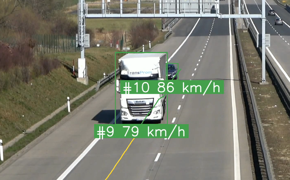
... video_info = sv.VideoInfo.from_video_path('autos.mp4') # initialize the dictionary that we are going to use to retailer the coordinates coordinates = defaultdict(lambda: deque(maxlen=video_info.fps)) for body in frame_generator: consequence = mannequin(body)[0] detections = sv.Detections.from_ultralytics(consequence) detections = byte_track.update_with_detections(detections=detections) factors = detections.get_anchors_coordinates( anchor=sv.Place.BOTTOM_CENTER) # plug the view transformer into an current detection pipeline factors = view_transformer.transform_points(factors=factors).astype(int) # retailer the remodeled coordinates for tracker_id, [_, y] in zip(detections.tracker_id, factors): coordinates[tracker_id].append(y) for tracker_id in detections.tracker_id: # wait to have sufficient information if len(coordinates[tracker_id]) > video_info.fps / 2: # calculate the velocity coordinate_start = coordinates[tracker_id][-1] coordinate_end = coordinates[tracker_id][0] distance = abs(coordinate_start - coordinate_end) time = len(coordinates[tracker_id]) / video_info.fps velocity = distance / time * 3.6 ...

Hidden Complexities with Pace Estimation

Many further components must be thought-about when constructing a real-world automobile velocity estimation system. Let’s briefly talk about a couple of of them.

Occluded and trimmed packing containers: The steadiness of the field is a key issue affecting the standard of velocity estimation. Small modifications within the measurement of the field when one automotive briefly obscures one other can result in giant modifications within the worth of the estimated velocity.

Setting a hard and fast reference level: On this instance, we used the underside middle of the bounding field as a reference level. That is attainable as a result of the climate circumstances within the video are good – a sunny day, no rain. Nonetheless, it’s simple to think about conditions the place finding this level will be way more troublesome.

The slope of the highway: On this instance, it’s assumed that the highway is totally flat. In actuality, this hardly ever occurs. To attenuate the impression of the slope, we should restrict ourselves to the half the place the highway is comparatively flat, or embrace the slope within the calculations.

Conclusion

There’s a lot extra you are able to do with velocity estimation. For instance, the under video reveals color-codes automobiles based mostly on automotive velocity. I hope this weblog put up will encourage you to construct one thing even cooler.

Keep updated with the initiatives we’re engaged on at Roboflow and on my GitHub! Most significantly, tell us what you’ve been capable of construct.