We created a Google Colab pocket book you can run in a separate tab whereas studying this weblog put up, permitting you to experiment and discover the ideas mentioned in actual time. Let’s dive in!
Introduction
Searching for a state-of-the-art object detector that you should utilize in an enterprise venture is tough. Hottest fashions include a license that forces you to open-source your complete venture. At the moment I will present you how you can practice an RTMDet – a mannequin that’s quick and correct sufficient to compete with high fashions, however which – as a consequence of its open license – you should utilize wherever.
What’s RTMDet?
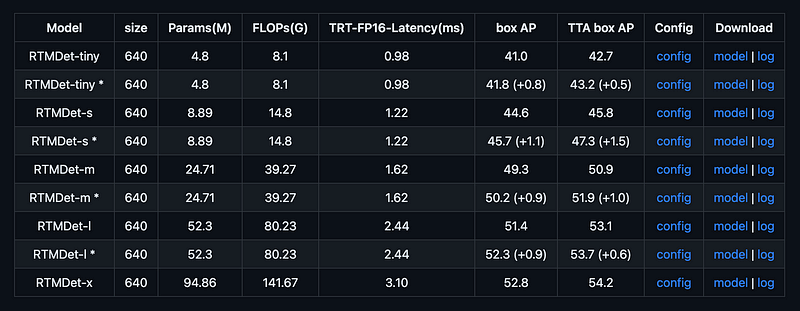
RTMDet is an environment friendly real-time object detector, with self-reported metrics outperforming the YOLO sequence. It achieves 52.8% AP on COCO with 300+ FPS on an NVIDIA 3090 GPU, making it one of many quickest and most correct object detectors out there as of scripting this put up.

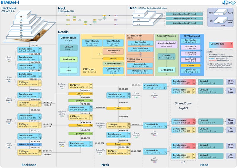
RTMDet makes use of an structure with appropriate capacities in each the spine and neck, constructed utilizing a fundamental constructing block comprising large-kernel depth-wise convolutions. This design enhances the mannequin’s skill to seize world context whereas sustaining quick inference pace.
Importantly, RTMDet is distributed by way of MMDetection and MMYOLO packages below the Apache-2.Zero license. Accuracy, pace, ease of deployment, and a permissive license make RTMDet a perfect mannequin for enterprise customers constructing industrial purposes.
What’s OpenMMLab?
OpenMMLab covers a variety of analysis subjects of pc imaginative and prescient, resembling classification, detection, segmentation, and super-resolution. A particular characteristic of this framework is that it’s divided into many libraries of restricted scope.

OpenMMLab has launched 30+ imaginative and prescient libraries, has carried out 300+ algorithms, and comprises 2000+ pre-trained fashions. All of the libraries have collected tens of 1000’s of stars on GitHub.
This tutorial will use 4 libraries from the OpenMMLab ecosystem:
- MMEngine — Foundational library for coaching deep studying fashions.
- MMCV — Foundational library for pc imaginative and prescient.
- MMDetection — Detection toolbox and benchmark.
- MMYOLO — YOLO sequence toolbox and benchmark. It provides state-of-the-art object detection fashions resembling YOLOv7, YOLOv8, PP-YOLOE, and RTMDet.
OpenMMLab Libraries Set up
Let’s begin by establishing the Python setting. MMYOLO depends on PyTorch, MMCV, MMEngine, and MMDetection.
When putting in PyTorch, make sure that to decide on a model that’s appropriate in your {hardware} and working system. A instrument on the official website will assist you compose the best set up command.

OpenMMLab has its personal bundle supervisor — MIM. Take a peek under for fast set up steps. Please seek advice from the Set up Information for extra detailed directions.
cd {HOME}
pip set up -U -q openmim
mim set up -q "mmengine>=0.6.0"
mim set up -q "mmcv>=2.0.0rc4,<2.1.0"
mim set up -q "mmdet>=3.0.0rc6,<3.1.0"
git clone https://github.com/open-mmlab/mmyolo.git
cd {HOME}/mmyolo
mim set up -v -e .
Lastly, let’s set up two extra Python libraries. roboflow— which we are going to use to obtain the dataset from Roboflow Universe. supervision— which can present us with utilities to visualise detections, load datasets, and benchmark the mannequin.
pip set up -q roboflow supervisionInference with Pre-trained RTMDet COCO mannequin
RTMDet structure is available in 5 totally different sizes: RTMDet-t, RTMDet-s, RTMDet-m, RTMDet-l, and RTMDet-x. All through this tutorial, we are going to use one of many bigger variations — RTMDet-l . Keep in mind that relying in your use case, your choice might differ. Take a peek at Determine 1. visualizing the speed-accuracy tradeoff.
After you have chosen the mannequin dimension you need to use, it’s time to obtain the suitable configuration file and pre-trained weights. You will discover the mandatory hyperlinks within the desk within the MMYOLO repository’s README. Obtain the correct information to your arduous drive and save them below the CONFIG_PATH and WEIGHTS_PATH paths.
import torch from mmdet.apis import init_detector DEVICE = torch.system('cuda:0' if torch.cuda.is_available() else 'cpu')
CONFIG_PATH = '...'
WEIGHTS_PATH = '...' mannequin = init_detector(CONFIG_PATH, WEIGHTS_PATH, system=DEVICE)
Now we’re able to initialize the mannequin. All we’ve got to do is name the init_detector operate out there in MMDetection API, offering it with CONFIG_PATH, WEIGHTS_PATH, and DEVICE as arguments. The worth of DEVICE will range relying in your {hardware} and the model of PyTorch you’ve gotten put in.
import cv2
import supervision as sv from mmdet.apis import inference_detector IMAGE_PATH = '...'
picture = cv2.imread(IMAGE_PATH) end result = inference_detector(mannequin, picture)
detections = sv.Detections.from_mmdetection(end result)
box_annotator = sv.BoxAnnotator()
annotated_image = box_annotator.annotate(picture.copy(), detections)
We are able to now use the mannequin to deduce any picture or video. We visualize the outcomes utilizing BoxAnnotator out there within the supervision library.

By default, the results of MMDetection inference appears chaotic. The mannequin returns a number of hundred proposed bounding packing containers. We should filter out detections based mostly on their confidence and use NMS to mix double-detections. We are able to do that by including one line of supervision code. I encourage you to learn extra concerning the superior detection filtering mechanisms out there in supervision.
import cv2
import supervision as sv from mmdet.apis import inference_detector IMAGE_PATH = '...'
picture = cv2.imread(IMAGE_PATH) end result = inference_detector(mannequin, picture)
detections = sv.Detections.from_mmdetection(end result)
detections = detections[detections.confidence > 0.3].with_nms()
box_annotator = sv.BoxAnnotator()
annotated_image = box_annotator.annotate(picture.copy(), detections)
Downloading a Dataset from Roboflow Universe
To coach a mannequin with the MMDetection framework, we want a dataset in COCO format. On this tutorial, I’ll use the football-player-detection dataset. Be at liberty to interchange it together with your dataset or one other dataset from Roboflow Universe.

For those who use a dataset from Roboflow Universe, export it in COCO-MMDetection format. This ensures clean integration within the coaching course of.
Another factor. If you wish to use your dataset however it isn’t in COCO format, no downside. You should use the supervision to transform it from PASCAL VOC or YOLO to COCO.
import roboflow roboflow.login()
rf = roboflow.Roboflow() WORKSPACE_NAME = "roboflow-jvuqo"
PROJECT_NAME = "football-players-detection-3zvbc"
PROJECT_VERSION = 2 venture = rf.workspace(WORKSPACE_NAME).venture(PROJECT_NAME)
dataset = venture.model(PROJECT_VERSION).obtain("coco-mmdetection")
Making ready Customized MMDetection Configuration File
Crafting a customized configuration file is essentially the most overwhelming side of the MMDetection framework.
The most effective technique is to repeat the uncooked configuration file of the mannequin you need to practice and make modifications. In my case, the unique configuration file for the RTMDet-l mannequin wanted a number of further necessary components.
Let’s begin by offering info on the dataset. Paths to the picture listing and annotation JSON for practice and validation subsets, in addition to the listing and variety of class names.
data_root = '.information/football-players-detection-2/' train_ann_file = 'practice/_annotations.coco.json'
train_data_prefix = 'practice/' val_ann_file = 'legitimate/_annotations.coco.json'
val_data_prefix = 'legitimate/' class_name = ('ball', 'goalkeeper', 'participant', 'referee')
num_classes = 4
As normal, we should outline typical coaching parameters: batch dimension, studying price, enter picture dimension, and epoch depend.
train_batch_size_per_gpu = 8
base_lr = 0.004
max_epochs = 50
img_scale = (640, 640)
Lastly, it’s a good suggestion to outline integration with Tensor Board or Weights & Biases.
_base_.visualizer.vis_backends = [
dict(type='LocalVisBackend'),
dict(type='TensorboardVisBackend'),]
Practice RTMDet and Analyze the Metrics
As soon as we’ve got an entire configuration file, many of the work is already behind us. All we’ve got to do is run the practice.py script and be affected person. The coaching time relies on the chosen mannequin structure, the scale of the dataset, and the {hardware} you’ve gotten.
cd {HOME}/mmyolo
python instruments/practice.py configs/rtmdet/customized.py
When the coaching ends, all artifacts might be saved within the mmyolo/work_dirs listing. There we are going to discover our mannequin’s weights and configuration file and, if we’ve got configured integration with Tensor Board, the logs that we will visualize. All we have to do is replace the tensorboard argument —-logdir in order that it results in the work_dirs related to the coaching job.

Evaluating the RTMDet Mannequin with Supervision
It’s good follow to judge the mannequin after the coaching. It will be significant to not benchmark the mannequin on pictures we beforehand used throughout coaching. The purpose is to check how effectively the mannequin will deal with pictures it has not seen earlier than.
The confusion matrix visualizes mannequin efficiency by evaluating its predicted classifications to precise floor fact values, highlighting true positives, false positives, true negatives, and false negatives. To do that, we are going to use the beforehand put in supervision pip bundle.
We load our dataset from the arduous drive, outline an inference callback (containing our educated mannequin), and are able to go.
IMAGES_DIRECTORY = f"{dataset.location}/check"
ANNOTATIONS_PATH = f"{dataset.location}/check/_annotations.coco.json" ds = sv.DetectionDataset.from_coco( images_directory_path=IMAGES_DIRECTORY, annotations_path=ANNOTATIONS_PATH,
) def callback(picture: np.ndarray) -> sv.Detections: end result = inference_detector(mannequin, picture) detections = sv.Detections.from_mmdetection(end result) detections = detections[detections.confidence > 0.3] return detections.with_nms(threshold=0.7) confusion_matrix = sv.ConfusionMatrix.benchmark( dataset = ds, callback = callback
)
confusion_matrix.plat()
Only one have a look at the confusion matrix provides us numerous details about our dataset and the mannequin educated with it. Our information set is extremely unbalanced — most annotations characterize the participant class. In distinction, our mannequin does effectively with detecting goalkeepers and gamers, poorly with referees, and badly with the ball.

Imply common precision (mAP) is one other metric typically used to benchmark object detection fashions. It enables you to describe the mannequin’s accuracy utilizing a single quantity between Zero and 1.
mean_average_precision = sv.MeanAveragePrecision.benchmark( dataset = ds, callback = callback
)
mean_average_precision.map50_95
Conclusion
We encourage you to make use of the Google Colab pocket book supplied, delve deeper into the configurations, and experiment with totally different mannequin architectures from the OpenMMLab ecosystem.